Nonsmooth and level-resolved dynamics illustrated with a periodically driven tight-binding model

Abstract

We point out that in the first-order time-dependent perturbation theory, the transition probability may behave nonsmoothly in time and have kinks periodically. Moreover, the detailed temporal evolution can be sensitive to the exact locations of the eigenvalues in the continuum spectrum, in contrast to coarse-graining ideas. Underlying this nonsmooth and level-resolved dynamics is a simple equality about the sinc function sinc x ≡ sin x/x. These physical effects appear in many systems with approximately equally spaced spectra, and are also robust for larger amplitude coupling beyond the domain of perturbation theory. We use a one-dimensional periodically driven tight-binding model to illustrate these effects, both within and outside the perturbative regime.

Main article text

INTRODUCTION

Coarse graining is a common trick in physics. In principle, it is invoked whenever one replaces a summation by an integral. The idea behind, which is justified for many purposes, is that structures too fine do not matter; what matter are the structures on a sufficiently large scale. A good example is calculating the heat capacity of a cloud of ideal gas. The exact single-particle eigenvalues of course depend on the specific shape and size of the container. However, for a macroscopic system, one does not need to know the spectrum to that precision at all. On the other hand, one just needs to know the number of states in a macroscopic energy interval. In other words, we can replace the real density of states, which consists of delta functions, by a coarse-grained one, which is a continuous and smooth function of energy. According to Weyl's law [1], the coarse-grained density of state is proportional to the volume of the container but independent of its shape. The problem is thus greatly simplified and we have shape-independent heat capacity.

Coarse graining is also used in the definition and derivation of the celebrated Fermi's golden rule [2, 3]. Suppose we have an unperturbed Hamiltonian, ${\widehat{H}}_0$, whose eigenvalues and eigenstates are denoted as E_n and |n〉. Let the system be in the state |i〉 initially and let a sinusoidal perturbation $\widehat{V}(t)=\mathcal{V}{e}^{i\omega t}+{\mathcal{V}}^{†}{e}^{-i\omega t}$ be turned on at t = 0. In the first-order time-dependent perturbation theory, Fermi's golden rule states that the transition rate from the initial state to the continuum band {|n〉} is given by (ħ = 1 in this paper):

(1) $$w_{i\to [n]}\equiv -\frac{dp}{dt}={2\pi \overline{|\langle n|\mathcal{V}|i\rangle {|}^2}\rho (E_n)|}_{E_n\simeq E_i\pm \omega }.$$

Here p(t) denotes the probability of the system remaining in the initial state. In this formula, coarse graining is used twice; the quantity ρ(E_n) is the coarse-grained density of states mentioned above, while $\overline{|\langle n|\mathcal{V}|i\rangle {|}^2}$ is the coarse-grained coupling strength. The coarse graining implies that the transition dynamics is smooth with respect to the driving frequency ω. To be specific, p(t) as a function of t should be largely invariant if the value of ω is changed on the scale of the level spacing of the spectrum {E_n}. Or, the transition dynamics cannot resolve the finest structure of the spectrum.

However, in this paper, we point out that while this presumption is true in a finite time interval, it may break down beyond some critical time (the Heisenberg time actually). Specifically, under some mild conditions, the function p(t) can be nonsmooth and have kinks periodically. In the regime where the first-order perturbation theory is valid, it is simply a piecewise linear function. Moreover, under the same perturbation, the trajectories of p(t) can bifurcate suddenly and significantly for two adjacent initial states. Similarly, for the same initial state, the trajectory of p(t) can be tuned to a great extent by changing the frequency ω on the scale of the level spacing. In one word, the transition dynamics can be nonsmooth and have a single-level resolution beyond some critical time. These effects can be demonstrated by using the one-dimensional tight-binding model as we shall do below.

We note that some similar nonsmoothness effect has been observed previously in the model of a single two-level atom interacting with a one-dimensional optical cavity [4–6]. However, those authors had a different perspective and their approaches were either purely numerical [4] or based on an exactly soluble model [5, 6]. In contrast, our approach will be based on the first-order perturbation theory and some simple mathematical properties of the sinc x ≡ sin x/x function. The perturbative approach means some new insight and it enables us to make predictions about a generic model, such as the one-dimensional tight-binding model. It also demonstrates that Fermi's golden rule can break down even in the first-order perturbation regime ($1-p\left(t\right)\ll 1$).

The rest of the paper is organized as follows. In the General Formalism Section, we derive the effect from the first-order perturbation theory, assuming that the energy levels in the target region are equally spaced and the couplings to them are equal too. The problem reduces to periodic sampling of the function sinc² x, which is to be solved in the An Equality of the Sinc² x Function Section using the Poisson summation formula. There we obtain a piecewise linear function of time, which is the essence of the effect. Then, in the Driven Tight-binding Model Section, we demonstrate the effect by taking two examples of tight-binding lattices and driving a local parameter (potential of a single site). In these realistic models, the two assumptions are only approximately satisfied, but we still see sharp kinks (nonsmooth behavior) and sudden bifurcations (level resolution). Moreover, all these effects persist even beyond the perturbative regime, i.e., for large amplitude driving.

GENERAL FORMALISM

Let us recall that in the first-order time-dependent perturbation theory, the probability of finding the system in states other than the initial state is given by Ref. [7]. (Although here in view of the demonstration in the Driven Tight-binding Model Section, we have assumed a sinusoidal perturbation, the formalism applies equally well to the case of a constant perturbation.):

(2) $$1-p(t)=4{\displaystyle \sum _{n\ne i}|\langle n|\mathcal{V}|i\rangle {|}^2\frac{{\sin }^2[(E_n-E_f)t/2]}{|E_n-E_f{|}^2}},$$

with E_f ≡ E_i + ω. Here we assume that stimulated absorption is the only dominant process. The case when stimulated absorption and stimulated radiation are dominant simultaneously can be treated equally well. Now we make two assumptions: (1) the level spacing E_n+1 − E_n and (2) the coupling strength $|\langle n|\mathcal{V}|i\rangle |$ are both slowly varying with respect to n for E_n ≃ E_f. We will discuss later for what kinds of model these assumptions are satisfied.

Under these assumptions, in view of the fact that the sinc² x function decays in the rate of |x|⁻² to zero as |x| → ∞, it is a good approximation to replace the real spectrum in Equation (2) by an equally spaced spectrum and the real couplings by a constant one. That is:

(3) $$1-p(t)\simeq 4g^2{\displaystyle \sum _{m\in \mathbb{Z}}\frac{{\sin }^2[({\tilde{E}}_m-E_f)t/2]}{|{\tilde{E}}_m-E_f{|}^2}}.$$

Here the pseudo-spectrum is defined as ${\tilde{E}}_m=E_{n^{*}}+m(E_{n^{*}+1}-E_{n^{*}})$, $m\in \mathbb{Z}$, and the constant coupling is $g=|\langle n^{*}|\mathcal{V}|i\rangle |$. The level |n^*〉 is chosen by the condition $E_{n^{*}}\le E_f<E_{n^{*}+1}$. Defining $\delta =E_{n^{*}+1}-E_{n^{*}}$ and $\alpha =(E_f-E_{n^{*}})/\delta$, we can rewrite Equation (3) as:

(4) $$1-p(t)\simeq \left(\frac{4g^2}{{\delta }^2}\right)W_{\alpha }(T)$$

Here, we have introduced the function of the rescaled dimensionless time T = δt/2:

(5) $$W_{\alpha }(T)\equiv T^2{\displaystyle \sum _{m\in \mathbb{Z}}{\text{sinc}}^2[(m-\alpha )T]},$$

which will be our primary concern. The summation means to sample the function sinc² x uniformly from −∞ to +∞ with an equal distance T. The offset is determined by α. Apparently, W_α = W_α+1 and because of the evenness of the sinc function, W_α = W_−α. Therefore, W_α is determined by its value in the interval of 0 ≤ α ≤ 1/2.

An equality of the sinc² x function

To carry out the summation in Equation (5), we employ the celebrated Poisson summation formula [8], which essentially means that periodically sampling a function in real space is equivalent to periodically sampling (with appropriate phase shifts) the same function in momentum space. To this end, we need the Fourier transform of sinc² x. Because it is the square of the function sinc x, in turn, we need the Fourier transform of sinc x, from which the Fourier transform of sinc² x can be calculated by convolution. But it is well known that sinc is the Fourier transform of the window function! That is, the function defined as:

(6) $$F_1(q)\equiv {\displaystyle {\int }_{-\infty }^{+\infty }dx{e}^{-iqx}\frac{\sin x}{x}},$$

which can be calculated by using complex contour integration, is:

(7) $$F_1(q)=\{\begin{array}{cc}\pi ,& \left|q\right|\le 1,\\ 0,& \left|q\right|>1.\end{array}$$

It has a finite support of [−1, +1] and has a constant value of π there, as illustrated in Figure 1a. By convolution, the Fourier transform of sinc² x is then:

(8) $$F_2(q)=\{\begin{array}{ll}\frac{\pi }{2}(2+q),\hfill & -2\le q\le 0,\hfill \\ \frac{\pi }{2}(2-q),\hfill & 0\le q\le +2,\hfill \\ 0,\hfill & \left|q\right|>2,\hfill \end{array}$$

which is a triangle function on the support [−2, +2] as illustrated in Figure 1b. We note that the fact that sinc² x has a finite support in the Fourier space is a consequence of the Paley–Wiener theorem [9]. The function is entire and is of exponential type 2. Therefore, by the Paley–Wiener theorem, its Fourier transform is supported on [−2, 2].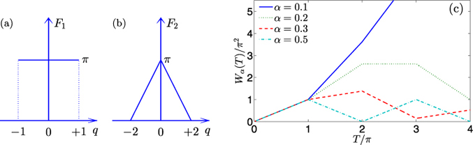

Figure 1.

(Color online) (a) Fourier transform of the function sinc x and (b) Fourier transform of its square sinc² x. The latter is calculated from the former by convolution. The point is that both have a finite support. In (c), the function W_α(T) [see Eqs. (5) and (10)], which is calculated by using the Poisson summation formula and the fact in (b), is displayed for four different values of the offset α. It is piecewise linear. In the interval of 0 ≤ T ≤ π, its value is independent of the parameter α; while beyond this interval, its value is very sensitive to α. Note that for α = 0.5, W_α returns to zero at T = 2mπ periodically; while for α = 0, W_α ∝ T² asymptotically.

Now by the Poisson summation formula, we have:

(9) $$W_{\alpha }(T)=T{\displaystyle \sum _{n\in \mathbb{Z}}{F}_2\left(\frac{2\pi n}{T}\right)\exp \left(-i2\pi n\alpha \right)}.$$

We have thus successfully converted the original, equally spaced sampling of sinc² x, into an equally spaced sampling of its Fourier transform F₂(q). Now the point is that, this function has only a finite support. This means for given T, only a finite number of terms on the right hand side of Equation (9) will contribute. In particular, if 0 < T ≤ π, only the n = 0 term is nonzero and we get W_α(T) = πT, which is simply linearly proportional to T. Moreover, it is independent of the parameter α. By Equation (4), we get 1 − p(t) ≃ (2πg²/δ)t for 0 ≤ t ≤ t_c ≡ 2π/δ. Here we note that the critical time t_c is the so-called Heisenberg time. This is nothing but Fermi's golden rule if one notes that 1/δ is the coarse-grained density of states.¹ The α-independence also justifies the coarse-graining usually employed.

However, more generally, if mπ < T ≤ (m + 1)π, the nonzero terms in the summation are −m ≤ n ≤ m. We have then (θ ≡ 2πα):

(10) $$W_{\alpha }(T)=\pi T{\displaystyle \sum _{n=-m}^m\exp (in\theta )}-{\displaystyle \sum _{n=1}^{m}2}{\pi }^{2}n\cos (n\theta ).$$

This is our central result. The function W_α is still linear on the interval [mπ, (m + 1)π], but now the slope depends on α and m, which means it is a piecewise linear, nonsmooth function of T and has kinks at T = mπ periodically. In Figure 1c, the function W_α(T) is plotted for four different values of α. We see that although on the interval (0, π), the lines all coincide, immediately after the first kink, they all split out and their late developments differ significantly. Therefore, we see that even in the first-order perturbation theory, Fermi's golden rule can break down beyond some critical time.

At this point, it should be clear why we need the two assumptions at the beginning. We need to sample the sinc² x function uniformly and with equal weight to make use of the nice expression (10). We argue that the two assumptions are satisfied for a generic model with only one degree of freedom, but are dissatisfied for a generic model with more than one degree of freedom. The reason is simply that if one adds up two arithmetic sequences with different common differences, one does not get an arithmetic sequence. Therefore, we have to admit that, the effects discussed in this paper are relevant only to single particle models in one dimension.

By Equation (4), the nonsmooth, α-dependent dynamics of W_α translates into that of p(t). Both the coupling g and the level spacing δ are slowly varying functions of E_i and ω. More specifically, they changes only negligibly if E_i or ω changes on the order of δ. However, α varies on the order of δ. Therefore, we expect that under the same sinusoidal perturbation, adjacent eigenstates generally will have significantly different transition dynamics beyond the critical time t_c. Or, if we start from the same initial state but drive with slightly different ω, the t > t_c dynamics has level resolution – it depends on the exact location of E_f relative to the eigenvalues.

DRIVEN TIGHT-BINDING MODEL

In the following, we take the one-dimensional tight-binding model to illustrate these effects. Consider a one-dimensional lattice with N = 2L + 1 sites and with periodic boundary condition. The Hamiltonian is:

(11) $${\widehat{H}}_{TBM}=-{\displaystyle \sum _{j=-L}^L({\widehat{a}}_j^{†}{\widehat{a}}_{j+1}+{\widehat{a}}_{j+1}^{†}{\widehat{a}}_j)}.$$

The eigenstates are labeled by the integer −L ≤ k ≤ L. The kth eigenstate is ${\psi }_k(n)=e^{i2\pi kn/N}/\sqrt{N}$ and the corresponding eigenvalue is ε_k = −2 cos(2πk/N). Suppose initially the particle is in the state ${\psi }_{k_i}$ and at t = 0 we start modulating the potential of site j = 0 sinusoidally by adding to the Hamiltonian (11) the term:

(12) $$\widehat{V}(t)=\Delta {\widehat{a}}_0^{†}{\widehat{a}}_0\sin \omega t.$$

The perturbation couples all the eigenstates with equal amplitude, i.e., $|\langle {\psi }_{k_2}|\mathcal{V}|{\psi }_{k_1}\rangle |=\Delta /2N$ for all k_1,2 (Here the perturbation couples not only the initial state and the continuum states, but also the continuum states themselves. In contrast, in the exactly soluble model in Refs. [4–6], there is no coupling between the continuum states. Of course, in the first-order perturbation, the coupling between the continuum states does not appear). We choose k_i such that the initial energy $E_i={ϵ}_{k_i}$ is close enough to the bottom of the energy band and we need only to consider the stimulated absorption process (see Figure 2a).

Figure 2.

(Color online) Two scenarios of transition in the periodically driven one-dimensional tight-binding model. (a) Continuum-to-continuum transition. The initial state is an eigenstate, i.e., a Bloch state, of the perfect model (11). (b) Bound-to-continuum transition. The unperturbed Hamiltonian (13) contains a defected site and the initial state is the defect mode. Note that locally speaking, the spectrum of the tight-binding model is almost equally spaced.

The two assumptions about the level spacings and couplings are satisfied. Let E_f = E_i + ω fall between ${ϵ}_{k_f}$ and ${ϵ}_{k_f+1}\left(k_f>0\right)$. We then approximate the real spectrum by the spectrum $\{{ϵ}_{k_f}+n({ϵ}_{k_f+1}-{ϵ}_{k_f})|n\in \mathbb{Z}\}$. We have thus for the parameters δ and g: $\delta ={ϵ}_{k_f+1}-{ϵ}_{k_f}$ and g = Δ/2N. The parameter α is then determined as $\alpha =(E_f-{ϵ}_{k_f})/({ϵ}_{k_f+1}-{ϵ}_{k_f})$. Both g and δ are slowly varying with respect to the index k_i. However, α is expected to be somewhat random, as demonstrated below. We can then use Equations (4) and (10) to predict the time evolution of p [but here we have to multiply the right hand side of Equation (10) by a factor of two because a generic level of Equation (11) is doubly degenerate] to the first-order of perturbation.

In Figure 3, we compare the approximate results obtained in this way with the results obtained by solving the time-dependent Schrödinger equation exactly. Therefore, we have taken a lattice of N = 601 sites and studied the transition dynamics of five successive plane waves, i.e., for 41 ≤ k_i ≤ 45, under the same driving. We see that when the driving amplitude Δ is small enough (Figure 3a), the exact evolution of p agrees with the approximation very well. The trajectories of p show kinks periodically and between the kinks, they are all linear. The trajectories all collapse into one before the first kink. However, immediately after the first kink they spread out, somewhat randomly in the sense that they are not ordered as their wave vectors. As the driving amplitude increases (Figure 3b and 3c), the exact result deviates from the approximate prediction gradually, and the kinks get rounded gradually, starting first with the later ones. However, even when the first-order perturbation is no longer good quantitatively in the regime 0 < t < t_c (see Figure 3c), the first kink still happens and we still observe the state-dependent spread-out. Moreover, the second kink is still visible for those trajectories with $p\lesssim 1$ marginally satisfied.

Figure 3.

(Color online) Probability of finding the particle in the initial Bloch state against the number of driving cycles. The lattice size is N = 601 and the period of driving is 2π/ω = 3. The amplitude of driving is shown in each panel. In each panel, five successive initial states, with 41 ≤ k_i ≤ 45 are studied. The solid lines are exact results obtained by solving the time-dependent Schrödinger equation, while the dotted lines are based on (4) and (10). In each panel, at ωt/2π = 200, from up to down, the solid lines correspond to k_i = 41, 43, 44, 45, 42, respectively. The same ordering holds for the dotted lines. Note that the distance between the kinks is independent of Δ.

As a second scenario, let us consider a one-site-defected tight-binding model. Now the Hamiltonian is (U > 0):

(13) $$\widehat{H}{\text{′}}_{\text{TBM}}=-{\displaystyle \sum _{j=-L}^{L-1}({\widehat{a}}_j^{†}{\widehat{a}}_{j+1}+{\widehat{a}}_{j+1}^{†}{\widehat{a}}_j)-U{\widehat{a}}_0^{†}{\widehat{a}}_0}.$$

The defect introduces a localized mode ϕ_d around it. For a sufficiently big L, its energy is $E_i=-\sqrt{U^2+4}$. Suppose initially the particle is trapped in this mode. Under the perturbation (12), it couples to the eigenstates in the continuum band (illustrated in Figure 2b). Note that the model (13) is symmetric with respect to the defected site and therefore all its eigenstates have a definite parity. In particular, the defect mode has an even parity. The perturbation (12) preserves the parity symmetry and therefore, it couples the defect mode only to those even-parity states.

Denote the even-parity eigenstates as ϕ_m and correspondingly, the eigenvalues as {ε_m}. Numerically, it is verified that the level spacing ε_m+1 − ε_m, as well as the coupling $|\langle {\varphi }_m|\mathcal{V}|{\varphi }_d\rangle |$, is slowly varying with respect to m. Let E_f = E_i + ω fall between ε_n and ε_n+1. As in the first example, we approximate the real spectrum by $\{{\epsilon }_n+m({\epsilon }_{n+1}-{\epsilon }_n)|m\in \mathbb{Z}\}$, which means δ = ε_n+1 − ε_n, and take g as $g=|\langle {\varphi }_n|\mathcal{V}|{\varphi }_d\rangle |$. Both δ and g are almost invariant when ω changes on the scale of δ. However, the parameter α = (E_f − ε_n)/δ can be changed significantly in this process.

Therefore, the transition dynamics might change substantially as ω changes on the scale of the mean level spacing of the model. This is indeed the case, as shown in Figure 4. Therefore, a relatively weak (Figure 4a) and a relatively strong driving case (Figure 4b) are studied. In both cases, three slightly different driving periods are considered. Like in Figure 3, we see periodic kinks and the spread-out of the trajectories at the first kink. In the stronger driving case, the exact trajectories no longer follow the predictions based on the approximation (they simply cannot, as the approximation predicts $p\ll 1$ at some point, which is inconsistent with the perturbation theory). The trajectories even look curved. However, the periodic kinks remain as the most apparent features.

Figure 4.

(Color online) Probability of finding the particle in the initial state (the defect mode) against the number of driving cycles. The lattice size is N = 201 and the depth of the defect is U = 1. The amplitude of driving is shown in each panel. In each panel, the solid lines are exact results obtained by solving the time-dependent Schrödinger equation, while the dashed lines are based on (4) and (10). In each panel, at ωt/2π = 100, from bottom to top, the solid lines correspond to 2π/ω = 2.5, 2.51, 2.52, respectively. The same ordering holds for the dashed lines. Note that the distance between the kinks is independent of Δ.

So far, our discussion is based on mathematics only. Here are some remarks from a physical point of view. First, the level resolution dynamics belongs to the long-time regime t > t_c = 2π/δ. This is consistent with the usual time-energy uncertainty relation – one has to wait a time on the order of 1/δ to have an energy resolution of δ. Second, the periodic kinks are a consequence of interference. The local driving generates some out-going waves. These waves are peaked in momentum space and travel along the lattice with a group velocity of:

(14) $$v_g\equiv \frac{dE}{dk}=\frac{\delta }{(2\pi /N)}=\frac{N\delta }{2\pi }.$$

In time N/v_g, which equals t_c, they come back to the perturbed site and interfere with the newly generated outgoing waves. This picture explains why in Figures 3 and 4 the kinks are robust even beyond the perturbative regime.

CONCLUSION AND DISCUSSION

In conclusion, we have reexamined the first-order time-dependent perturbation theory. By noticing some simple analytic equality about the sinc function, we predicted that under some mild conditions, the probability of finding the system in its initial state is a piecewise linear function of time. The slope of the line changes periodically with the period being inversely proportional to the level spacing of the spectrum. These predictions were confirmed in the one-dimensional tight-binding model. Although the predictions are based on the first-order time-dependent perturbation theory, the signatures persist even outside of the perturbative regime.

It should be worthwhile to construct some system to observe the predicted effects experimentally. A potential scheme is to use guiding photonic structures [10]. By the quantum-optics analogy, the Hamiltonians (11) and (13), as well as the time-varying driving (12), can all be readily realized. The driving does not need to be sinusoidal actually, it can equally well be in the periodic square form, which is experimentally more feasible. The main difficulty might come from the relatively large number of sites required for a clean manifestation of the effects.

Acknowledgment

We are grateful to André Eckardt, Hua-Tong Yang, Hui Jing, Michael Sekania, and Alex D. Gottlieb for helpful discussions.

References

1. Strauss WA. Partial differential equations: an introduction, 2nd ed. Hoboken (NJ): John Wiley & Sons; 2008.

2. Dirac PAM. The quantum theory of the emission and absorption of radiation. Proc R Soc Lond A. 1927;114:243–265. [Cross Ref]

3. Fermi E. Nuclear physics. Chicago (IL): University of Chicago Press; 1950.

4. , , , , . Cavity-modified spontaneous emission: from Rabi oscillations to exponential decay. Phys Rev A. 1996;53:2816–21. [Cross Ref]

5. , . Decay of quantum states in some exactly soluble models. Physica. 1972;60(1):1–26. [Cross Ref]

6. , . The calculated photon: visualization of a quantum field. Am J Phys. 2002;70:58. [Cross Ref]

7. , . Modern quantum mechanics, 2nd ed. San Francisco (CA): Pearson; 2011.

8. Grafakos L. Classical Fourier analysis, 2nd ed. New York (NY): Springer-Verlag; 2008.

9. Rudin W. Real and complex analysis, 3rd ed. New York: McGraw-Hill; 1987.

10. Longhi S. Quantum-optical analogies using photonic structures. Laser Photon Rev. 2009;3:243–261. [Cross Ref]

Competing Interests

The authors declare no competing interests.

Publishing Notes

© 2014 Jiang Min Zhang and M. Haque. This work has been published open access under Creative Commons Attribution License CC BY 4.0, which permits unrestricted use, distribution, and reproduction in any medium, provided the original work is properly cited. Conditions, terms of use and publishing policy can be found at www.scienceopen.com.

Footnotes

¹

Pedagogically, this approach of deriving Fermi's golden rule, although not as general as, has some advantage over the conventional one in textbooks like Ref. [7], in the sense that the Dirac delta function is not invoked.